Rift Inversion Results Figures
This notebook uses the GDTchron results from process_riftinversion.ipynb to create a figure and video showing the results. Note that it relies on that previous notebook having access to large source files, and so it is not reproducible without a local copy of the model results
[1]:
import os
import shutil
import warnings

import cmcrameri.cm as cmc
import cv2
import matplotlib.cm as cm
import matplotlib.colors as mcolors
import matplotlib.pyplot as plt
import numpy as np
import pandas as pd
import pyvista as pv
from IPython.display import Video
from tqdm import tqdm

import gdtchron as gdt

plt.rcParams['pdf.fonttype'] = 42
This cell sets an environment variable that is necessary for transparency to render correctly when plotting the strain over the composition from the model
[2]:
os.environ['GALLIUM_DRIVER'] = 'softpipe'
This cell gathers the paths to the original model files for plotting composition, strain rate, and temperature
[3]:
# Get full output files from local source
sol_path = (
    'solution'
)
files = [
    os.path.join(sol_path, file) for file in os.listdir(sol_path)
    if file.endswith('.pvtu')
]
files.sort()
The cell below sets up parameters for the figure.
[4]:
directory_tchron = 'meshes_tchron'
time1 = 20  # Ma
time2 = 0  # Ma

model_step = 0.1

step1 = int((36 - time1) / model_step)
step2 = int((36 - time2) / model_step)

file1 = files[step1]
file2 = files[step2]

file1_tchron = os.path.join(directory_tchron, 'meshes_tchron_160.vtu')
file2_tchron = os.path.join(directory_tchron, 'meshes_tchron_360.vtu')

colors = ['#66CCEE', '#BBBBBB', '#EE6677', '#228833']
cmap = mcolors.ListedColormap(colors)

opaque_cm = cmc.lapaz_r
cm_strain = 'inferno_r'
cat_cmap = cmc.batlowS

opacity_strain = [0, 0.8, 0.8, 0.8, 0.8]
lim_strain = [0, 5]

lim_tchron = [0, 36]  # Ma

bounds = [250, 750, -20, 150]  # km, X position and depth
bounds_ahe = [250, 750, -15, 70]  # km, 2x vertical exaggeration
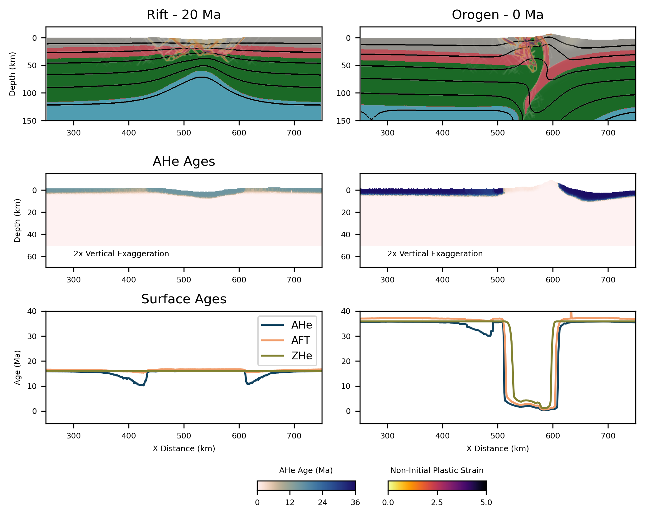
The cell below makes the figure, which includes comparison of the structure of the model with the predicted thermochronometric ages
[5]:
fig, axs = plt.subplots(3, 2, dpi=300, figsize=(7, 5))

axs = axs.flatten()

axs[0].set_title('Rift - 20 Ma', fontsize=10)
axs[1].set_title('Orogen - 0 Ma', fontsize=10)

axs[2].set_title('AHe Ages', loc='center', fontsize=10)

mesh1 = pv.read(file1)
mesh1.points /= 1e3  # Convert m to km
mesh1['T'] -= 273.15  # Convert temp to °C
mesh1.points[:, 1] = -(mesh1.points[:, 1] - 600)  # Convert Y position to depth

mesh2 = pv.read(file2)
mesh2.points /= 1e3  # Convert m to km
mesh2['T'] -= 273.15  # Convert temp to °C
mesh2.points[:, 1] = -(mesh2.points[:, 1] - 600)  # Convert Y position to depth

mesh1_tchron = pv.read(file1_tchron)
mesh1_tchron.points /= 1e3  # Convert m to km
# Convert Y position to depth
mesh1_tchron.points[:, 1] = -(mesh1_tchron.points[:, 1] - 600)

mesh2_tchron = pv.read(file2_tchron)
mesh2_tchron.points /= 1e3  # Convert m to km
# Convert Y position to depth
mesh2_tchron.points[:, 1] = -(mesh2_tchron.points[:, 1] - 600)

mesh1 = gdt.add_comp_field(mesh1)
mesh2 = gdt.add_comp_field(mesh2)

mesh1_cntrs = mesh1.contour(isosurfaces=np.arange(200, 1600, 200), scalars='T')
mesh2_cntrs = mesh2.contour(isosurfaces=np.arange(200, 1600, 200), scalars='T')

gdt.plot_vtk_2d(mesh1, 'comp_field', bounds=bounds, ax=axs[0],
           cmap=cmap)

gdt.plot_vtk_2d(mesh2, 'comp_field', bounds=bounds, ax=axs[1],
            cmap=cmap)

gdt.plot_vtk_2d(mesh1_cntrs, None, bounds=bounds, ax=axs[0],
          color='black', line_width=5, colorbar=True)

gdt.plot_vtk_2d(mesh2_cntrs, None, bounds=bounds, ax=axs[1],
            color='black', line_width=5, colorbar=True)

gdt.plot_vtk_2d(mesh1, 'noninitial_plastic_strain', bounds=bounds, ax=axs[0],
          cmap=cm_strain, opacity=opacity_strain, clim=lim_strain)

gdt.plot_vtk_2d(mesh2, 'noninitial_plastic_strain', bounds=bounds, ax=axs[1],
          cmap=cm_strain, opacity=opacity_strain, clim=lim_strain)

gdt.plot_vtk_2d(mesh1_tchron, 'AHe', bounds=bounds_ahe, ax=axs[2],
            cmap=opaque_cm, colorbar=False, clim=lim_tchron,
               vertical_exaggeration=2)

gdt.plot_vtk_2d(mesh2_tchron, 'AHe', bounds=bounds_ahe, ax=axs[3],
            cmap=opaque_cm, colorbar=False, clim=lim_tchron,
               vertical_exaggeration=2)

axs[2].text(300, 60, '2x Vertical Exaggeration', fontsize=6)
axs[3].text(300, 60, '2x Vertical Exaggeration', fontsize=6)

x1 = np.round(mesh1_tchron.points[:, 0], 0)
x2 = np.round(mesh2_tchron.points[:, 0], 0)
He1 = mesh1_tchron['AHe']
He2 = mesh2_tchron['AHe']

AFT1 = mesh1_tchron['AFT']
AFT2 = mesh2_tchron['AFT']

ZHe1 = mesh1_tchron['ZHe']
ZHe2 = mesh2_tchron['ZHe']

df1 = pd.DataFrame({'x': x1, 'AHe': He1, 'AFT': AFT1, 'ZHe': ZHe1})
df1_max = df1.groupby('x').agg({'x': 'first', 'AHe': 'max', 'AFT': 'max', 'ZHe': 'max'})
df2 = pd.DataFrame({'x': x2, 'AHe': He2, 'AFT': AFT2, 'ZHe': ZHe2})
df2_max = df2.groupby('x').agg({'x': 'first', 'AHe': 'max', 'AFT': 'max', 'ZHe': 'max'})

axs[0].set_ylabel('Depth (km)', fontsize=6)
axs[2].set_ylabel('Depth (km)', fontsize=6)

axs[4].plot(df1_max['x'], df1_max['AHe'], c=cat_cmap.colors[6], label='AHe')
axs[4].plot(df1_max['x'], df1_max['AFT'], c=cat_cmap.colors[4], label='AFT')
axs[4].plot(df1_max['x'], df1_max['ZHe'], c=cat_cmap.colors[2], label='ZHe')

axs[4].legend(fontsize=8)

axs[5].plot(df2_max['x'], df2_max['AHe'], c=cat_cmap.colors[6])
axs[5].plot(df2_max['x'], df2_max['AFT'], c=cat_cmap.colors[4])
axs[5].plot(df2_max['x'], df2_max['ZHe'], c=cat_cmap.colors[2])

axs[4].set_xlim(250, 750)
axs[5].set_xlim(250, 750)
axs[4].set_ylim(40, -5)
axs[5].set_ylim(40, -5)
axs[4].set_title('Surface Ages', fontsize=10)
axs[4].set_ylabel('Age (Ma)', fontsize=6)
axs[4].set_xlabel('X Distance (km)', fontsize=6)
axs[5].set_xlabel('X Distance (km)', fontsize=6)

for ax in axs:
    ax.tick_params(axis='both', which='major', labelsize=6)
    ax.invert_yaxis()

plt.tight_layout()

cax_ahe = fig.add_axes([0.4, -0.05, 0.15, 0.02])
norm = mcolors.Normalize(vmin=lim_tchron[0], vmax=lim_tchron[1])
sm_ahe = cm.ScalarMappable(cmap=opaque_cm, norm=norm)
cax_ahe.tick_params(labelsize=6)
plt.colorbar(sm_ahe, cax=cax_ahe, orientation='horizontal')
cax_ahe.set_title('AHe Age (Ma)', fontsize=6)
cax_ahe.set_xticks([0, 12, 24, 36])

cax_strain = fig.add_axes([0.6, -0.05, 0.15, 0.02])
norm = mcolors.Normalize(vmin=lim_strain[0], vmax=lim_strain[1])
sm_strain = cm.ScalarMappable(cmap=cm_strain, norm=norm)
cax_strain.tick_params(labelsize=6)
plt.colorbar(sm_strain, cax=cax_strain, orientation='horizontal')
cax_strain.set_title('Non-Initial Plastic Strain', fontsize=6)
cax_strain.set_xticks([0, 2.5, 5])

fig.savefig('riftvsinv.pdf', bbox_inches='tight')
2026-02-09 15:14:36.280 ( 2.466s) [ 7B0D00A84740]vtkXOpenGLRenderWindow.:1458 WARN| bad X server connection. DISPLAY=
[6]:
# Create video - image creation
warnings.filterwarnings("ignore", category=UserWarning)

image_dir = 'images/'

try:
    shutil.rmtree(image_dir)
except Exception:
    print("Creating new image directory...")
else:
    print("Cleared existing image directory...")

os.makedirs(image_dir, exist_ok=False)

for k, file in enumerate(tqdm(files)):
    fig = plt.figure(dpi=300, figsize=(6.5, 4))

    ax0 = fig.add_subplot(221)
    ax1 = fig.add_subplot(222)
    ax2 = fig.add_subplot(212)
    axs = [ax0, ax1, ax2]

    tchron_file = os.path.join(
        directory_tchron, 'meshes_tchron_' + str(k).zfill(3) + '.vtu'
        )

    time = str(round(36 - (k * model_step), 1)) + ' Ma'
    time_file = str(round(k * model_step, 1)).zfill(4).replace('.', '-')

    axs[0].set_title(time, loc='left')

    mesh = pv.read(file)
    mesh.points /= 1e3  # Convert m to km
    mesh['T'] -= 273.15  # Convert temp to °C
    mesh.points[:, 1] = -(mesh.points[:, 1] - 600)  # Convert Y position to depth

    mesh_tchron = pv.read(tchron_file)
    mesh_tchron.points /= 1e3  # Convert m to km
    # Convert Y position to depth
    mesh_tchron.points[:, 1] = -(mesh_tchron.points[:, 1] - 600)

    mesh = gdt.add_comp_field(mesh)

    mesh_cntrs = mesh.contour(isosurfaces=np.arange(200, 1600, 200), scalars='T')

    gdt.plot_vtk_2d(mesh, 'comp_field', bounds=bounds, ax=axs[0],
               cmap=cmap)

    gdt.plot_vtk_2d(mesh_cntrs, None, bounds=bounds, ax=axs[0],
          color='black', line_width=5, colorbar=True)

    gdt.plot_vtk_2d(mesh, 'noninitial_plastic_strain', bounds=bounds, ax=axs[0],
              cmap=cm_strain, opacity=opacity_strain, clim=lim_strain)

    gdt.plot_vtk_2d(mesh_tchron, 'AHe', bounds=bounds_ahe, ax=axs[1],
            cmap=opaque_cm, colorbar=False, clim=lim_tchron,
                   vertical_exaggeration=2)

    x = np.round(mesh_tchron.points[:, 0], 0)
    AHe = mesh_tchron['AHe']
    AFT = mesh_tchron['AFT']
    ZHe = mesh_tchron['ZHe']

    df = pd.DataFrame({'x': x, 'AHe': AHe, 'AFT': AFT, 'ZHe': ZHe})
    df_max = df.groupby('x').agg(
        {'x': 'first', 'AHe': 'max', 'AFT': 'max', 'ZHe': 'max'}
        )

    axs[2].plot(df_max['x'], df_max['AHe'], c=cat_cmap.colors[6], label='AHe')
    axs[2].plot(df_max['x'], df_max['AFT'], c=cat_cmap.colors[4], label='AFT')
    axs[2].plot(df_max['x'], df_max['ZHe'], c=cat_cmap.colors[2], label='ZHe')

    axs[0].set_ylabel('Depth (km)', fontsize=6)

    axs[1].set_title('AHe')

    cax_ahe = fig.add_axes([0.7, 0.72, 0.15, 0.02])
    norm = mcolors.Normalize(vmin=0, vmax=36)
    sm = cm.ScalarMappable(cmap=opaque_cm, norm=norm)
    plt.colorbar(sm, cax=cax_ahe, orientation='horizontal')

    cax_ahe.set_xticks([0, 36])
    cax_ahe.tick_params(axis='both', which='major', labelsize=6)
    cax_ahe.set_title('AHe Age (Ma)', fontsize=6, pad=2)

    axs[2].set_xlim(250, 750)
    axs[2].set_ylim(40, -2)
    axs[2].set_title('Surface Ages', fontsize=10)
    axs[2].set_ylabel('Maximum Age (Ma)', fontsize=6)
    axs[2].legend(fontsize=6, loc='lower left')

    for ax in axs:
        ax.tick_params(axis='both', which='major', labelsize=6)
        ax.set_xlabel('X Distance (km)', fontsize=6)
        ax.invert_yaxis()

    plt.tight_layout()
    fig.savefig(image_dir + time_file + '.jpg')
    plt.close()
Creating new image directory...
100%|██████████| 361/361 [54:06<00:00, 8.99s/it]
[9]:
# Make movie
img_paths = [
    image_dir + file for file in sorted(os.listdir(image_dir)) if file.endswith('.jpg')
]

frame = cv2.imread(img_paths[0])
height, width, layers = frame.shape

fourcc = cv2.VideoWriter_fourcc(*'avc1')

frate = 1 / model_step

video = cv2.VideoWriter('video_riftinversion.mp4', fourcc, frate, (width, height))

for img in img_paths:
    video.write(cv2.imread(img))

cv2.destroyAllWindows()
video.release()
[10]:
video_path = 'video_riftinversion.mp4'
Video(video_path, embed=True, width=500)
[10]: